LoRA 介绍

本文旨在结合原文与Peft源码，介绍LoRA

读懂本文需：

• 熟悉Transformer结构

• 熟悉Pytorch、Python3

英文出自LoRA原文，源码出自Peft（删掉部分源码以便阅读）。如本博文存在疏漏，烦请e-mail联系作者

原文提出LoRA（Low-Rank Adaptation）方法，冻结预训练模型权重，将可训练的秩分解矩阵注入到Transformer，大大减少了用于下游任务的可训练参数数量。

We propose Low-Rank Adaptation, or LoRA, which freezes the pretrained model weights and injects trainable rank decomposition matrices into each layer of the Transformer architecture, greatly reducing the number of trainable parameters for downstream tasks

LoRA原理

LoRA相较Prompt或Prefix Tuning，需更改网络结构（保留原网络参数）。它的目标对象是Dense层，翻译原文：

神经网络中的Dense层参数矩阵一般是满秩。研究表明，作用在特定领域（downtask）时，这些参数矩阵具有低的“内在维度”，即使随机映射到较小的子空间，仍可高效推理。微调的目的往往是将神经网络作用于特定任务，LoRA作者假设在Adaptation过程中，权重矩阵更新后也具有较低的“内在秩”。

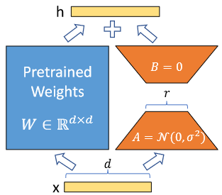
对预训练模型参数$W_0 \in \mathbb{R}^{d\times k}$，通过低秩分解的更新参数：$\ W_0 + \Delta W = W_0 + BA$，其中$B\in \mathbb{R}^{d \times r}$，$A \in \mathbb{R}^{r \times k}$，秩$r\ll\min(d,k)$。微调时冻结$W_0$，仅用梯度下降更新$A$和$B$中的可训练参数。$W_0$和$BA$处理相同的输入数据，最后输出的向量坐标逐项相加。

引入LoRA前递推公式为：

$$h=W_0x$$

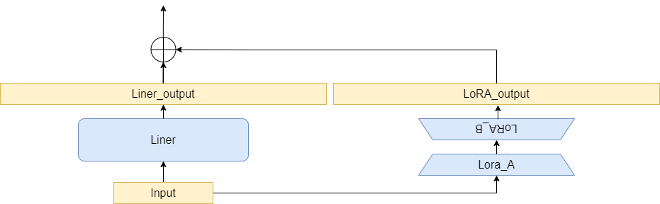
引入LoRA后递推公式为：

$$h=W_0x+\Delta Wx=W_0 + BAx$$

引入系数$\frac{\alpha}{r}$对$\Delta W x$进行缩放，$\alpha$是秩$r$的一个constant。梯度下降时，调整$\alpha$的方式和调整学习率$lr$类似，$\alpha$作用是在改变$r$值时减少超参数调参过程。

We then scale $\Delta W x$ by $\frac{\alpha}{r}$ , where $\alpha$ is a constant in $r$. When optimizing with Adam, tuning α is roughly the same as tuning the learning rate if we scale the initialization appropriately.

引入$\alpha$系数后，递推公式为：

$$h=W_0x+\frac{\alpha}{r}\Delta Wx=W_0 + \frac{\alpha}{r}BAx$$

新增参数位置

原则上可以将LoRA应用于神经网络中任何权重矩阵子集。

In principle, we can apply LoRA to any subset of weight matrices in a neural network to reduce the number of trainable parameters

以原文默认情况为例：将LoRA仅作用于自注意力相关的参数（Self-Attention）

We limit our study to only adapting the attention weights for downstream tasks and freeze the MLP modules (so they are not trained in downstream tasks) both for simplicity and parameter-efficiency.

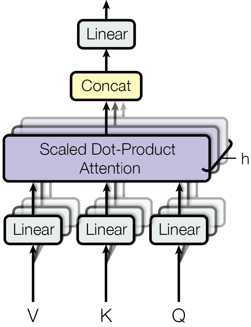
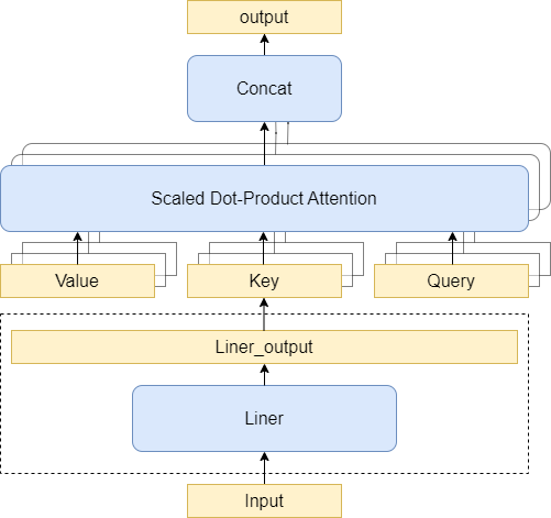
在Peft的实现中，LoRA作用于线性层和一维卷积层（linear/Conv1D）。本博文LoRA作用于Self-Attention层的query、key、value的映射权重矩阵（query_key_value），即Transformer原文中的$W_q,W_k,W_v$。对应下图Transformer的Self-Attention结构中的三个线性层：

Transformer/Bloomz将$W_q,W_k,W_v$三个参数矩阵用单个线性层统一实现，再将Linear层的输出拆分成三个向量，作为$Attention$层的输入，Multi-Head也在拆分时进行。如下图所示

引入LoRA时不必单独为$W_q,W_k,W_v$单独设计通路和参数，仅需在Linear层新增一个LoRA旁路（上图虚线位置）

参数插入方式

# peft/tuners/lora/layer.py
# line 720
new_module = Linear(target, adapter_name, **kwargs)

• Linear：它不是Pytorch的Linear，而是Peft重写的带LoRA旁路的Linear
• target：被替换的神经网络层，此处为nn.Linear
• kwargs：包含LoRA的参数：内在秩$r$及缩放系数$\alpha$

Linear层的初始化过程如下：

# peft/tuners/lora/layer.py
# line 191
class Linear(nn.Module, LoraLayer):
    # Lora implemented in a dense layer
    def __init__(
        self,
        base_layer,
        r: int = 0,
        lora_alpha: int = 1,
        lora_dropout: float = 0.0,
        **kwargs,
    ) -> None:
        super().__init__()
        LoraLayer.__init__(self, base_layer, **kwargs)
        self.update_layer(adapter_name, r, lora_alpha, lora_dropout, init_lora_weights, use_rslora)

初始化新Linear的重要步骤有两个

• LoraLayer.__init__(self, base_layer, **kwargs)：将原先的layer作为该Linear对象的base_layer

• self.update_layer(adapter_name, r, lora_alpha, lora_dropout, init_lora_weights, use_rslora)：设置LoraLayer的LoRA参数

① LoraLayer层的初始化方式

# peft/tuners/lora/layer.py
# line 31
class LoraLayer(BaseTunerLayer):
    def __init__(self, base_layer: nn.Module, **kwargs) -> None:
        self.base_layer = base_layer
        self.r = {}
        self.lora_alpha = {}
        self.lora_A = nn.ModuleDict({})
        self.lora_B = nn.ModuleDict({})
        self.kwargs = kwargs

        base_layer = self.get_base_layer()
        if isinstance(base_layer, nn.Linear):
            in_features, out_features = base_layer.in_features, base_layer.out_features
            
        self.in_features = in_features
        self.out_features = out_features

• self.base_layer = base_layer：将原先的Dense层作为新Linear的线性层
• in_features, out_features = base_layer.in_features, base_layer.out_features：获取原先Dense层的输入维度和输出维度，存储用于后续的LoRA参数矩阵$B$和$A$的shape设置。

② LoRA矩阵的分配及参数设置

class LoraLayer(BaseTunerLayer):
    # peft/tuners/lora/layer.py
    # line 76
    def update_layer(self, adapter_name, r, lora_alpha, lora_dropout, init_lora_weights, use_rslora):
        self.r[adapter_name] = r
        self.lora_A[adapter_name] = nn.Linear(self.in_features, r, bias=False)
        self.lora_B[adapter_name] = nn.Linear(r, self.out_features, bias=False)
        if use_rslora:
            self.scaling[adapter_name] = lora_alpha / math.sqrt(r)
        else:
            self.scaling[adapter_name] = lora_alpha / r
            
        if init_lora_weights == "loftq":
            self.loftq_init(adapter_name)
        elif init_lora_weights:
            self.reset_lora_parameters(adapter_name, init_lora_weights)

• 展示$A\in \mathbb{R}^{in\_features \times r}$（源码中为self.lora_A）及$B\in \mathbb{R}^{r \times out\_features}$（源码中为self.lora_B）
• self.reset_lora_parameters(adapter_name, init_lora_weights)用于$W_A,W_B$​的初始化
• self.scaling[adapter_name] = lora_alpha / r：根据$\alpha$及$r$计算缩放系数

③ LoRA矩阵的默认初始化方式

class LoraLayer(BaseTunerLayer):
    # peft/tuners/lora/layer.py
    # line 114
    def reset_lora_parameters(self, adapter_name, init_lora_weights):
        if adapter_name in self.lora_embedding_A.keys():
        # initialize a the same way as the default for nn.linear and b to zero
            nn.init.zeros_(self.lora_embedding_A[adapter_name])
            nn.init.normal_(self.lora_embedding_B[adapter_name])

• nn.init.zeros_(self.lora_embedding_A[adapter_name])：$A\in \mathbb{R}^{in\_features \times r}$（源码中为self.lora_A）初始为0
• nn.init.normal_(self.lora_embedding_B[adapter_name])：$B\in \mathbb{R}^{r \times out\_features}$​​用标准正态分布初始化

默认初始化方式和LoRA原文正好相反（见图1），原文”使用随机高斯分布初始化$A$，$B$设为0，因此$\Delta W=BA$在训练伊始是0"

We use a random Gaussian initialization for $A$ and zero for $B$, so $\Delta W=BA$ is zero at the beginning of training.

前向传播方式

前向传播源码如下：

class Linear(nn.Module, LoraLayer):
    # peft/tuners/lora/layer.py 
    # line 301    
    def forward(self, x: torch.Tensor, *args: Any, **kwargs: Any) -> torch.Tensor:
        previous_dtype = x.dtype

        if self.disable_adapters:
            if self.merged:
                self.unmerge()
            result = self.base_layer(x, *args, **kwargs)
        elif self.merged:
            result = self.base_layer(x, *args, **kwargs)
        else:
            result = self.base_layer(x, *args, **kwargs)
            for active_adapter in self.active_adapters:
                if active_adapter not in self.lora_A.keys():
                    continue
                lora_A = self.lora_A[active_adapter]
                lora_B = self.lora_B[active_adapter]
                dropout = self.lora_dropout[active_adapter]
                scaling = self.scaling[active_adapter]
                x = x.to(lora_A.weight.dtype)
                result += lora_B(lora_A(dropout(x))) * scaling

        result = result.to(previous_dtype)
        return result

关注源码中的两行：

• result = self.base_layer(x, *args, **kwargs) ：原线性层仍执行前向传播流程
• result += lora_B(lora_A(dropout(x))) * scaling：和公式保持一致

写在后面

LoRA作者强调不会引入推理时延：只需要用$W^{\prime}=W+BA$替换原有参数$W$，由于$W^{\prime}$和$W$维度相同，因此前向传播执行矩阵乘法时，时间复杂度一致，不会引入推理时延。工程实践中，如果不采用$W^{\prime}$替换$W$（由self.merged控制），$BAx$会执行两次矩阵乘法，此时会引入了理时延。

另一点，作者提到一些微调方法会减少模型的有效sequnece length，这一点博主会补充在《prompt tuning介绍》一文。

reduce the model’s usable sequence length

参考

1. Attention Is All You Need
2. LoRA: Low-Rank Adaptation of Large Language Models
3. huggingface/transformers
4. huggingface/peft